Fiji Plugins
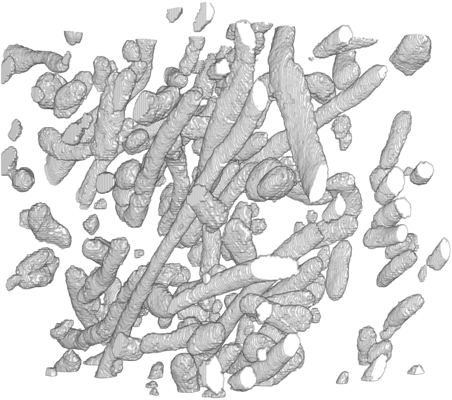
The code provided on this web page is for segmenting mitochondria in 3d EM datasets.
We also provide instructions on how to use the code as well as an EM dataset that can be used to train and test the algorithm.
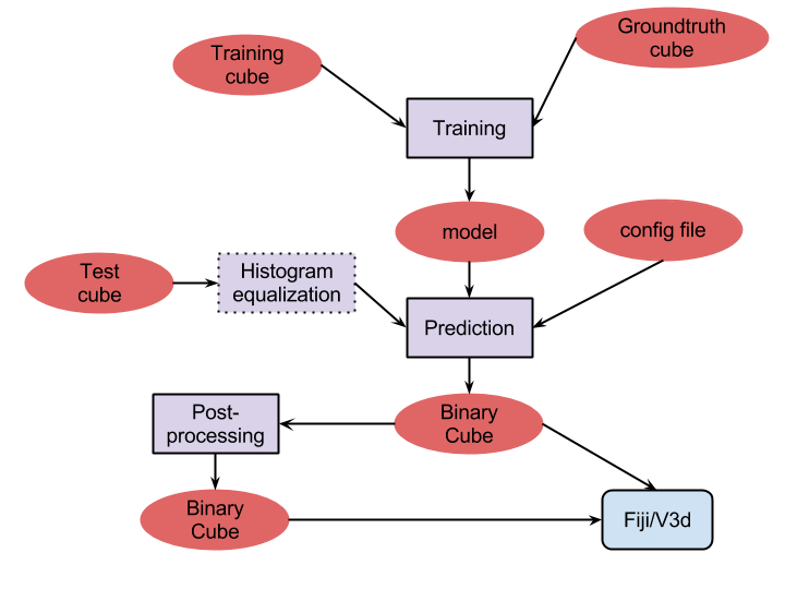
The diagram below gives an overview of the segmentation process that consists of two to four steps. First, the system has to be trained to recognize mitochondria. This training step will generate a model file that will be used in the prediction step of the segmentation. The prediction step will then generate a binary TIF cube that can be loaded in Fiji or v3d. Alternatively, one can also post-process the cube to remove small components that are expected to be false detections. Note that if your test cube looks fairly different from the training cube, an additional step (e.g. histogram equalization) might be required.
Installation & Execution
- Download plugin
- Start fiji (recommended running fiji for heavy duty operations) [1]
./fiji -Xms10g -Xmx10g -Xincgc -XX:MaxPermSize=256m -XX:PermSize=256m -XX:NewRatio=5 -XX:CMSTriggerRatio=50 -XX:+UseCompressedOops — - Install plugin
- Run CVLab SSVM plugin (fiji’s plugin section)
- Change configuration file with the path of your ground truth/images
- Train
- Choose model & Predict
Generating ground-truth data for training
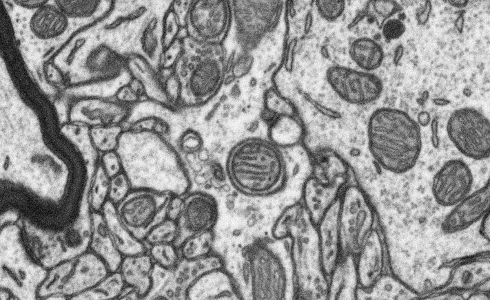
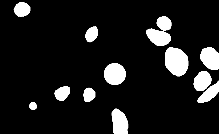
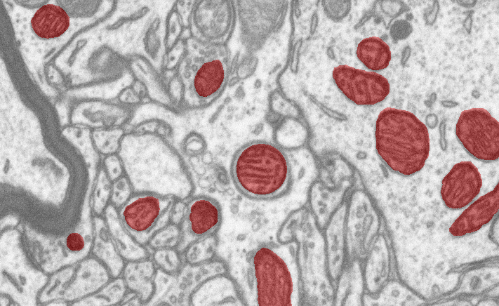
Our algorithm requires a ground-truth volume where the instances of the object you want to detect are marked as illustrated on the above figure. The path of this ground-truth volume will have to be specified in the configuration file during training (see maskTrainingDir argument described in the training section).
When labelling the ground-truth, we strongly advise to pick a sub-volume with difficult cases (cluster of vesicles, regions containing clutter, weirdly-shaped mitochondria,…). You have to make sure that your training set is representative of the test set, which means that you should include all kind of mitochondria.
An improperly trained algorithm will likely miss some mitochondria whose appearance is too different from the ones included in the training set. Another common mistake is the false detection of clusters of vesicles. Including these hard examples in your training set will almost surely lead to better results.
Configuration
The program relies on a configuration file that contains all the parameters needed for training or applying the algorithm to a new dataset. Below is a description of each parameter.
- trainingDir
- Input volume (TIF cube).
- maskTrainingDir
- Mask volume (TIF cube or series of png images containing black and white voxels only)
- outputModel
- Output model file (default=model.txt)
- testDir
- Test input volume (TIF cube).
- maskTestDir
- Test mask volume (TIF cube containing black and white voxels only).
- stepForOutputFiles
- output files and corresponding scores are computed every stepForOutputFiles iterations. Reasonable values are 10 for default training algorithm and 100 for stochastic optimization (-w 9 option described below).
- featureTypes
- Type of features extracted from the image/cube and used to train a model. featureTypes should be either 1 (histograms) or 33 (histograms and rays).
- Ray feature parameters
- Reasonable values are provided in the default configuration file at the bottom of this page but tuning these values will most likely be necessary if you intend to use the ray features.
- nMaxIterations
- Maximum number of iterations. This number should be around 500-1000 iterations depending on how much training data is provided to the algorithm.
An example configuration file named config.txt with a set of default parameters is provided for convenience.
Datasets
The dataset available for download on this webpage represents a 5x5x5µm section taken from the CA1 hippocampus region of the brain, corresponding to a 1065x2048x1536 volume. The resolution of each voxel is approximately 5x5x5nm. The data is provided as multipage TIF files that can be loaded in Fiji.
Embed of video is only possible from Mediaspace, Vimeo or Youtube
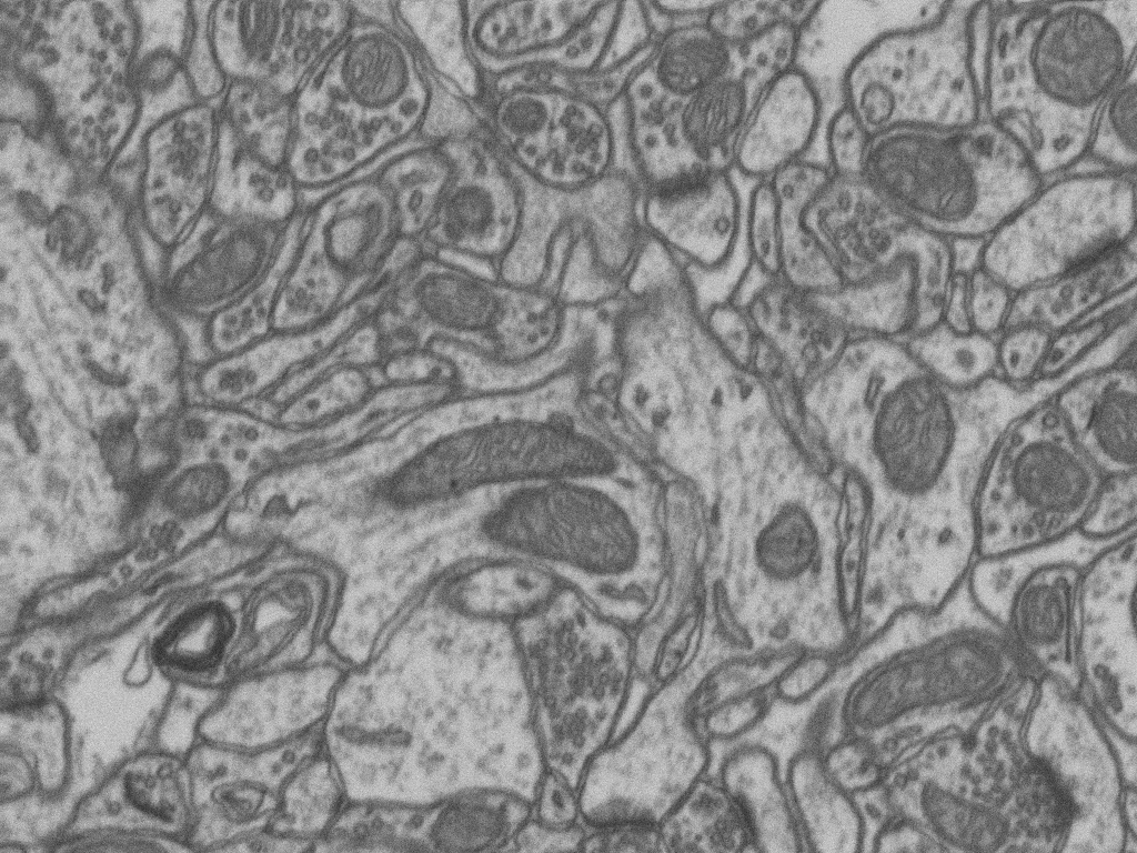
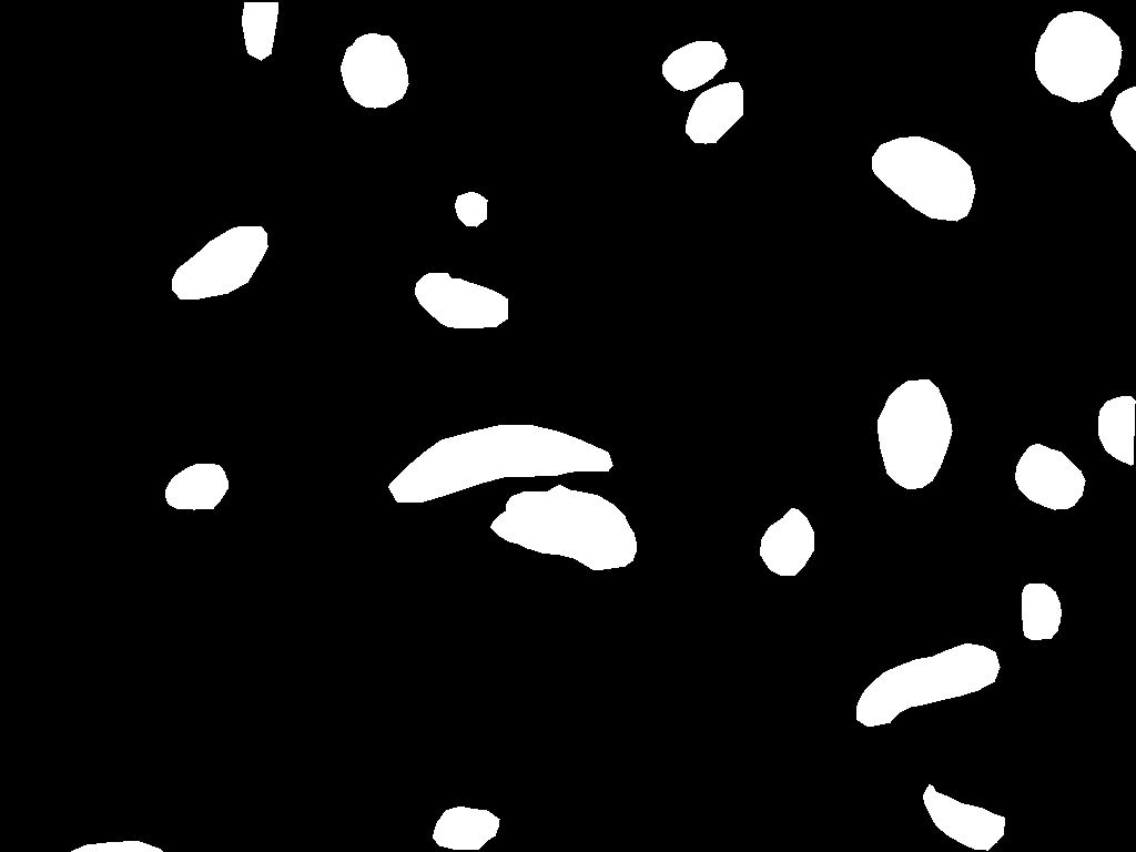
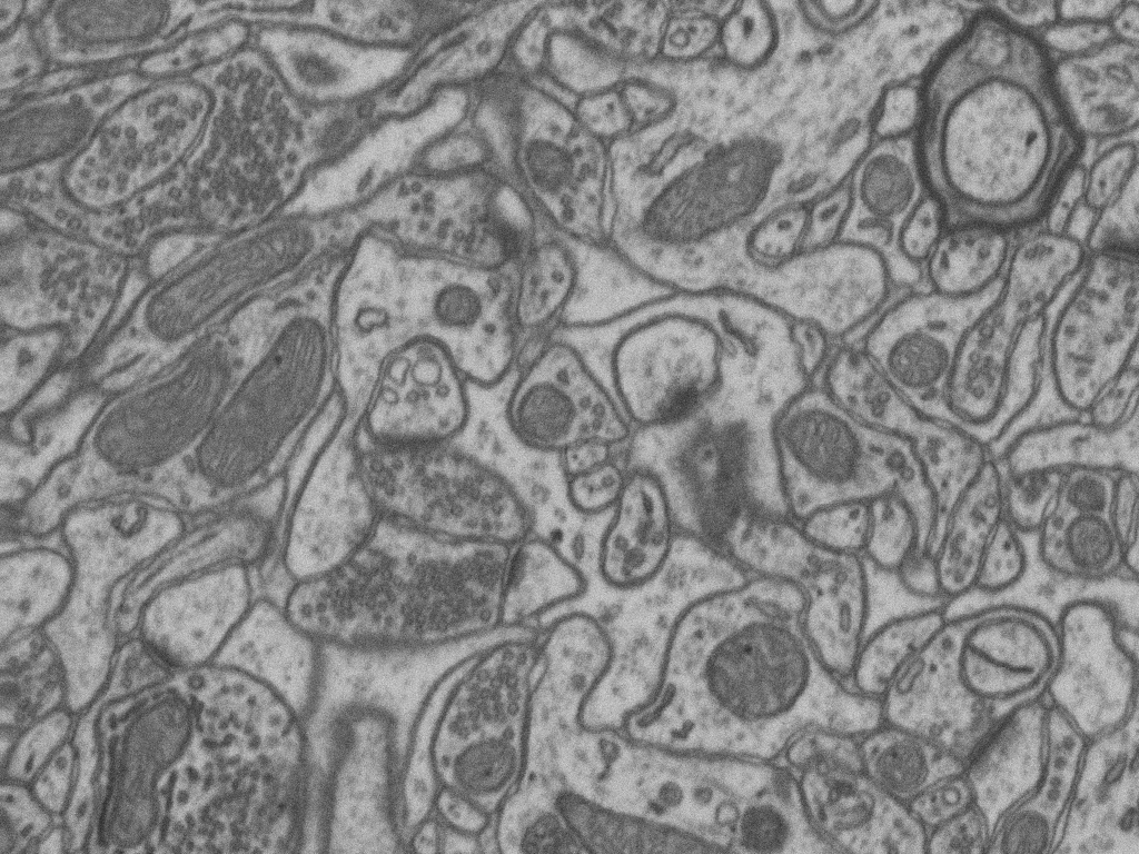
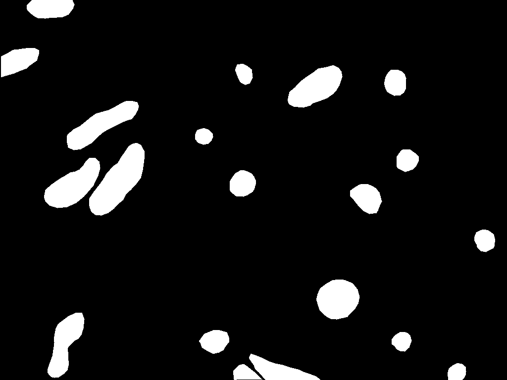
We annotated mitochondria in two sub-volumes. Each sub-volume consists of the first 165 slices of the 1065x2048x1536 image stack. The volume used for training our algorithm in the publications mentionned at the bottom of this page is the top part while the bottom part was used for testing.
Although our line of research was primarily motivated by the need to accurately segment mitochondria and synapses, other structures are of interest for neuroscientists such as vesicles or cell boundaries. This dataset was acquired by Graham Knott and Marco Cantoni at EPFL. It is made publicly available in the hope of encouraging similar sharing of useful data amongst researchers and also accelerating neuroscientific research.
For further information, please visit http://www.epfl.ch/labs/cvlab/research/medical/em/mitochondria.
References
Please note that the publication lists from Infoscience integrated into the EPFL website, lab or people pages are frozen following the launch of the new version of platform. The owners of these pages are invited to recreate their publication list from Infoscience. For any assistance, please consult the Infoscience help or contact support.
Learning for Structured Prediction Using Approximate Subgradient Descent with Working Sets
2013. Conference on Computer Vision and Pattern Recognition (CVPR), Portland, Oregon, USA, June 23-28, 2013. DOI : 10.1109/Cvpr.2013.259.Please note that the publication lists from Infoscience integrated into the EPFL website, lab or people pages are frozen following the launch of the new version of platform. The owners of these pages are invited to recreate their publication list from Infoscience. For any assistance, please consult the Infoscience help or contact support.
Supervoxel-Based Segmentation of Mitochondria in EM Image Stacks with Learned Shape Features
IEEE Transactions on Medical Imaging. 2012. Vol. 31, num. 2, p. 474-486. DOI : 10.1109/TMI.2011.2171705.License
The source code is available upon request for academic purposes only and is distributed under a proprietary non-commercial license. If you are interested in using this algorithm in a commercial product, you can contact us to purchase a commercial license.
Contact
Please mail [email protected] or [email protected] for bug reports, comments and questions.
Download
Fiji plugins of Lucchi
Frequently Asked Questions
Why are files created in the training and test directories?
The files created in the training and test directory are results of some precomputations (for the image features, supervoxels, …) that are re-loaded the next time you run the algorithm which significantly speeds things up.